Perceiver: General Perception with Iterative Attention

2021

Perceiver: General Perception with Iterative Attention

Andrew Jaegle, Felix Gimeno, Andrew Brock, and 3 more authors

Jun 2021

Paper Abstract

Biological systems perceive the world by simultaneously processing high-dimensional inputs from modalities as diverse as vision, audition, touch, proprioception, etc. The perception models used in deep learning on the other hand are designed for individual modalities, often relying on domain-specific assumptions such as the local grid structures exploited by virtually all existing vision models. These priors introduce helpful inductive biases, but also lock models to individual modalities. In this paper we introduce the Perceiver - a model that builds upon Transformers and hence makes few architectural assumptions about the relationship between its inputs, but that also scales to hundreds of thousands of inputs, like ConvNets. The model leverages an asymmetric attention mechanism to iteratively distill inputs into a tight latent bottleneck, allowing it to scale to handle very large inputs. We show that this architecture is competitive with or outperforms strong, specialized models on classification tasks across various modalities: images, point clouds, audio, video, and video+audio. The Perceiver obtains performance comparable to ResNet-50 and ViT on ImageNet without 2D convolutions by directly attending to 50,000 pixels. It is also competitive in all modalities in AudioSet.

@misc{2103.03206v1,
  author = {Jaegle, Andrew and Gimeno, Felix and Brock, Andrew and Zisserman, Andrew and Vinyals, Oriol and Carreira, Joao},
  title = {Perceiver: General Perception with Iterative Attention},
  eprint = {2103.03206},
  archiveprefix = {arXiv},
  primaryclass = {cs.CV},
  year = {2021},
  month = jun,
  url = {https://arxiv.org/abs/2103.03206},
  file = {perceiver.pdf},
  eprintnover = {2103.03206}
}

Three Important Things

1. Cross-Attention Bottleneck for Efficient Input Processing

One of the key innovations in the Perceiver is the introduction of a cross-attention module. In traditional attention mechanisms, applying the attention operation directly to large-scale inputs, such as images or audio signals, can be computationally expensive. The complexity of self-attention grows quadratically with the size of the input.

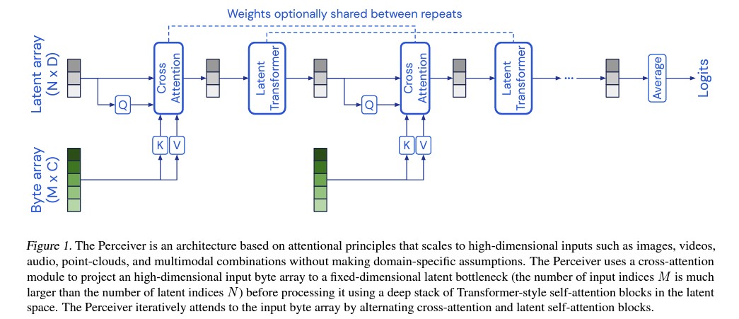
The Perceiver tackles this by projecting the input data (such as pixel arrays from images or audio samples) into a much smaller latent array via a cross-attention mechanism. This cross-attention module allows the model to summarize the input into a smaller set of latent vectors, which are then processed by a Transformer. The cross-attention module’s complexity is reduced from quadratic (O(M²)) to linear (O(MN)), where M is the size of the input array, and N is the size of the latent array.

This bottlenecking mechanism allows the Perceiver to handle very large datasets efficiently without sacrificing performance.

2. Deep Transformer Network on Latent Space

After the cross-attention module maps the input into a lower-dimensional latent space, the Perceiver uses a deep Transformer to further process these latent representations. Unlike architectures like Vision Transformers (ViT) that operate directly on the pixel space, the Perceiver performs self-attention only within the latent space.

The latent Transformer has a complexity of O(N²), which is much smaller than the complexity of processing high-dimensional input data directly. By decoupling input size from the depth of the Transformer, the architecture can scale much deeper. For example, in their experiments, the authors built models with up to 48 Transformer layers without becoming computationally prohibitive.

To reduce the overall number of parameters and prevent overfitting, the Perceiver architecture uses weight sharing between the different layers of the Transformer blocks. This recurrent-like approach enables the same cross-attention and Transformer layers to be applied repeatedly, unrolling the model in depth.

This technique provides two benefits:

Reduced Parameter Count: Weight sharing can result in a 10x reduction in parameters compared to non-weight-shared models.
Improved Generalization: Sharing weights helps the model generalize better on unseen data by reducing overfitting. The architecture essentially operates like an RNN but processes input repeatedly rather than over time.

A Glaring Deficiency

Lack of Explicit Spatial Understanding

Despite its strengths, one of the most glaring deficiencies of the Perceiver architecture is its inherent lack of spatial inductive bias. Traditional CNNs, by design, capture spatial hierarchies using convolutions that operate over local neighborhoods in images. This means CNNs naturally understand how nearby pixels relate to one another, making them effective at capturing spatial relationships and patterns.

In contrast, the Perceiver treats the input as an unordered set of bytes without explicitly leveraging spatial or temporal structure. While position encodings (such as Fourier features) are used to inject positional information, they don’t provide the same level of inductive bias as CNNs. For tasks where spatial locality is critical (e.g., image processing), the Perceiver’s reliance on learned relationships between pixels may result in less effective feature extraction compared to CNN-based models.

Conclusion

The Perceiver architecture marks a significant step forward in handling large-scale and multimodal datasets. Its cross-attention mechanism for input compression and efficient processing in latent space makes it a powerful alternative to traditional models like CNNs and Vision Transformers. However, its generality comes at a cost: the lack of inherent spatial understanding limits its applicability to certain tasks.

Despite this, the Perceiver holds promise for applications requiring general, scalable models capable of handling diverse input types, including audio, images, and video. The model’s flexibility and ability to process large-scale data while keeping computational costs manageable make it an exciting development in the field of machine learning architectures.

2021